
On page 110 of Professor Stewart’s Casebook of Mathematical Mysteries, he shows a neat visual way of calculating the GCD (Greatest common denominator, aka HCF, Highest common factor. Given a box with sides of two different lengths, draw squares from the lesser side until you can draw no more. Then continue from the corner the other direction. The smallest square has edge length of the GCD!
This is of course equivalent to the usual algorithm you may have learned: Take two numbers, put the remainder of division below it, repeat while you can:
34
12
10
2
0 (no remainder – so the GCD of 34 and 12 is 2.
The example on the Wikipedia article only calls this a “visualization” and unfortunately doesn’t have the code for their example file shown:

So, let’s break this out into steps:
- Draw a rectangle mxn
- Draw lines every n. On the last one, change direction.
- Draw lines every (m/n remainder)… repeat.
We can call the movement to the right direction (1,0) direction, the movement up (0,1) direction. Multiplying one of these can move in that direction. We can plot a line using the plot function and the x and y points. For example the outer rectangle would be:
plt.plot([0,0,m,m,0],[0,n,n,0,0], '.-k')given all the x and y values separately.
So we want a recursive function that starts at a given point and goes a direction drawing lines until the end… When there is a remainder, going along the other direction and drawing lines the other way (the same draw procedure but with smaller numbers):
#!/usr/bin/env python
# -*- coding: utf-8 -*-
import matplotlib.pyplot as plt

def plot(plt,start,direction,sidelen,outer):
    n=0
    #move n along the line and then plot along the OTHER direction:
    if direction == [0,1]:
        plotting = [1,0]
    else:
        plotting = [0,1]
    #(x,y) start point, plus direction * length.
    while n<outer:
        x1=start[0]
        y1=start[1]
        x2=x1+plotting[0]*sidelen
        y2=y1+plotting[1]*sidelen
        print( 'Plotting (%s,%s) to (%s,%s)' % (x1,y1, x2,y2) )
        plt.plot([x1,x2],[y1,y2],'.-k')
        n = n + sidelen
        start[0] += sidelen*direction[0]
        start[1] += sidelen*direction[1]
    if n>outer:
        print('switching')
        #overshot, not evenly dividing. Last one:
        n = n - sidelen
        plot(plt,[x1,y1],plotting,outer-n,sidelen)
    else:
        print('%s evenly divides %s, done!' % (sidelen, outer))


def main(args):
    print('Enter 2 numbers')
    m = int(input())
    n = int(input())
    plt.plot([0,0,m,m,0],[0,n,n,0,0], '.-k')
    plot(plt,[0,0],[1,0], n, m)
    plt.axis('equal') #Make squares look square, rather than fitting all in view.
    plt.show()
if __name__ == '__main__':
    import sys
    sys.exit(main(sys.argv))
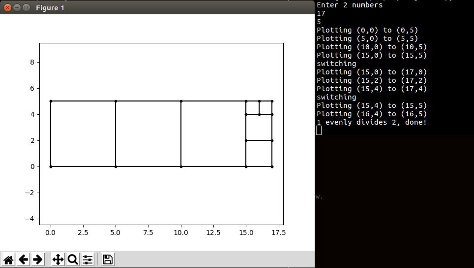
This gives an example doodle like in the book:
Now we can quickly and easily explore these with any numbers we care to graph. The next page of the book notes that “Lamé proved that the algorithm runs most slowly when m and n are consecutive members of the fibonacci sequence”. This is interesting, and if you try some of these you will see the pattern. Now you may be thinking, can we try plotting multiple of these in one file, or do plotting from Python command line? This is not hard, let’s just separate the rectangle plotting function from the main() that runs when you run the file:
#!/usr/bin/env python
# -*- coding: utf-8 -*-
import matplotlib.pyplot as plt

def plot(plt,start,direction,sidelen,outer):
    n=0
    #move n along the line and then plot along the OTHER direction:
    if direction == [0,1]:
        plotting = [1,0]
    else:
        plotting = [0,1]
    #(x,y) start point, plus direction * length.
    while n<outer:
        x1=start[0]
        y1=start[1]
        x2=x1+plotting[0]*sidelen
        y2=y1+plotting[1]*sidelen
        print( 'Plotting (%s,%s) to (%s,%s)' % (x1,y1, x2,y2) )
        plt.plot([x1,x2],[y1,y2],'.-k')
        n = n + sidelen
        start[0] += sidelen*direction[0]
        start[1] += sidelen*direction[1]
    if n>outer:
        print('switching')
        #overshot, not evenly dividing. Last one:
        n = n - sidelen
        plot(plt,[x1,y1],plotting,outer-n,sidelen)
    else:
        print('%s evenly divides %s, done!' % (sidelen, outer))

def plotRectangle(plt,m,n, startpoint):
    plt.plot([0,0,m,m,0],[0,n,n,0,0], '.-k')
    plot(plt,startpoint,[1,0], n, m)
    plt.axis('equal') #Make squares look square, rather than fitting all in view.

def main(args):
    print('Enter 2 numbers')
    m = int(input())
    n = int(input())
    plotRectangle(plt,m,n,[0,0])
    plt.show()
if __name__ == '__main__':
    import sys
    sys.exit(main(sys.argv))
Now you may wonder what that “__name__ == ‘__main__'” part of the code is doing, that lets the file both run the code when called directly, and be used just for its functions if you import it from the command line. Since I saved this as rectangle.py, I can open a Python console in the same directory (cd directoryname) and import the file and use it to plot wherever I want, from the console:
Python 3.5.2 (default, Jul 10 2019, 11:58:48)
[GCC 5.4.0 20160609] on linux
Type "help", "copyright", "credits" or "license" for more information.
>>>
>>> import matplotlib.pyplot as plt
>>> import rectangles
>>> rectangles.plotRectangle(plt,13,21,[0,0])
Plotting (0,0) to (0,21)
switching
Plotting (0,0) to (13,0)
Plotting (0,13) to (13,13)
switching
Plotting (0,13) to (0,21)
Plotting (8,13) to (8,21)
switching
Plotting (8,13) to (13,13)
Plotting (8,18) to (13,18)
switching
Plotting (8,18) to (8,21)
Plotting (11,18) to (11,21)
switching
Plotting (11,18) to (13,18)
Plotting (11,20) to (13,20)
switching
Plotting (11,20) to (11,21)
Plotting (12,20) to (12,21)
1 evenly divides 2, done!
>>> rectangles.plotRectangle(plt,34,55,[40,0])
Plotting (40,0) to (40,55)
switching
Plotting (40,0) to (74,0)
Plotting (40,34) to (74,34)
switching
Plotting (40,34) to (40,55)
Plotting (61,34) to (61,55)
switching
Plotting (61,34) to (74,34)
Plotting (61,47) to (74,47)
switching
Plotting (61,47) to (61,55)
Plotting (69,47) to (69,55)
switching
Plotting (69,47) to (74,47)
Plotting (69,52) to (74,52)
switching
Plotting (69,52) to (69,55)
Plotting (72,52) to (72,55)
switching
Plotting (72,52) to (74,52)
Plotting (72,54) to (74,54)
switching
Plotting (72,54) to (72,55)
Plotting (73,54) to (73,55)
1 evenly divides 2, done!
>>> plt.show()
which shows the following, odd looking visualization:
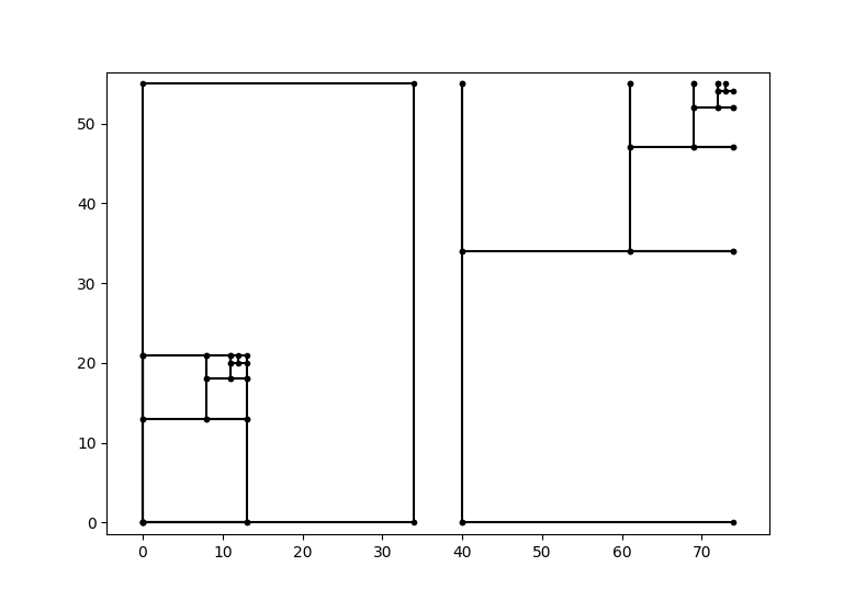
Oops! Note that though we added an option of where to start drawing this on the x/y plane, the rectangle draw at the start has not been adjusted. With a small adjustment to add the start value instead of starting at 0, that will properly draw it:
#!/usr/bin/env python
# -*- coding: utf-8 -*-
import matplotlib.pyplot as plt

def plot(plt,start,direction,sidelen,outer):
    n=0
    #move n along the line and then plot along the OTHER direction:
    if direction == [0,1]:
        plotting = [1,0]
    else:
        plotting = [0,1]
    #(x,y) start point, plus direction * length.
    while n<outer:
        x1=start[0]
        y1=start[1]
        x2=x1+plotting[0]*sidelen
        y2=y1+plotting[1]*sidelen
        print( 'Plotting (%s,%s) to (%s,%s)' % (x1,y1, x2,y2) )
        plt.plot([x1,x2],[y1,y2],'.-k')
        n = n + sidelen
        start[0] += sidelen*direction[0]
        start[1] += sidelen*direction[1]
    if n>outer:
        print('switching')
        #overshot, not evenly dividing. Last one:
        n = n - sidelen
        plot(plt,[x1,y1],plotting,outer-n,sidelen)
    else:
        print('%s evenly divides %s, done!' % (sidelen, outer))

def plotRectangle(plt,m,n, startpoint):
    #x,y start:
    xstart = startpoint[0]
    ystart = startpoint[1]
    plt.plot([xstart,xstart,xstart+m,xstart+m,xstart],[ystart,ystart+n,ystart+n,ystart,ystart], '.-k')
    plot(plt,startpoint,[1,0], n, m)
    plt.axis('equal') #Make squares look square, rather than fitting all in view.

def main(args):
    print('Enter 2 numbers')
    m = int(input())
    n = int(input())
    plotRectangle(plt,m,n,[0,0])
    plt.show()
if __name__ == '__main__':
    import sys
    sys.exit(main(sys.argv))
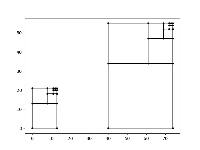
Note that we plotted the larger consecutive Fibonacci to the right, where you can see that the smaller is actually contained in it! When you think about it, visualizing the consecutive Fibonacci series will be equivalent to adding a square on that is the sum of the last two, so it makes sense that these will all look similar in that there is one square that can be clipped off each time. That’s why there will be a lot of steps in using division and remainders to calculate the GCD with Euler’s method.